深入理解 DDPM

DDPM，全称为 Diffusion Denoising Probability Models（扩散去噪概率模型），是一种生成模型，用于生成高质量的数据样本，如图像、音频或文本。这种方法的核心思想是模拟数据生成的逆向扩散过程，通过逐步去除噪声来生成数据样本。DDPM的工作原理可分为两个主要阶段：正向扩散（加噪）和逆向扩散（去噪）。本文将主要从数学角度详细剖析这两个过程。

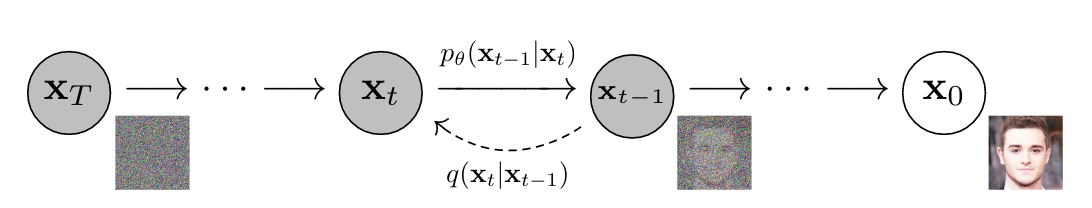
正向加噪过程

对 \(t\) 时刻的图像，其正向加噪过程可以由以下公式描述： \[ x_t = \sqrt{\alpha_t} x_{t - 1} + \sqrt{1 - \alpha_t} \epsilon_t \] \(\alpha_t\)（\(0 < \alpha_t < 1\)）在这里表示 \(t\) 时刻的加噪系数，是一个超参，随着 \(t\) 的增加，\(\alpha_t\) 会越来越小。\(\epsilon_t\) 是一个高斯噪音，服从标准正态分布。

根据上式，我们将 \(x_{t - 1}\) 递归展开，可以得到 \(x_t\) 和 \(x_{t - 2}\) 之间的关系： \[ x_t = \sqrt{\alpha_t}(\sqrt{\alpha_{t - 1}}x_{t - 2} + \sqrt{1 - \alpha_{t - 1}}\epsilon_{t - 1}) + \sqrt{1 - \alpha_t} \epsilon_t \] 整理可得： \[ x_t = \sqrt{\alpha_t \alpha_{t - 1}}x_{t - 2} + \sqrt{\alpha_t - \alpha_t\alpha_{t - 1}}\epsilon_{t - 1} + \sqrt{1 - \alpha_t}\epsilon_t \] 由于 \(\epsilon_t\) 和 \(\epsilon_{t - 1}\) 是两个独立且服从标准正态分布的随机变量，因此可以得到： \[ \sqrt{\alpha_t - \alpha_t\alpha_{t - 1}}\epsilon_{t - 1} + \sqrt{1 - \alpha_t}\epsilon_t \sim N(0, {(\sqrt{\alpha_t - \alpha_t\alpha_{t - 1}}\ )} ^ 2 + {(\sqrt{1 - \alpha_t}\ )} ^ 2) \] 即： \[ \sqrt{\alpha_t - \alpha_t\alpha_{t - 1}}\epsilon_{t - 1} + \sqrt{1 - \alpha_t}\epsilon_t \sim N(0, 1 - \alpha_t\alpha_{t - 1}) \] 因此原式可以改写为： \[ x_t = \sqrt{\alpha_t\alpha_{t - 1}}x_{t - 2} + \sqrt{1 - \alpha_t\alpha_{t - 1}}\epsilon \] 其中，\(\epsilon \sim N(0, 1)\)，这一步叫做重参数化。由数学归纳法，易证： \[ x_t = \sqrt{\bar{\alpha_t}}x_0 + \sqrt{1 - \bar{\alpha_t}}\epsilon \] 其中，\(\bar{\alpha_t} = \prod_{i = 1} ^ t \alpha_i\)，\(\epsilon \sim N(0, 1)\)。也就是说，从 \(t = 0\) 时刻加噪得到 \(t = x\) 时刻的图像，只需要一次随机采样即可。

多次加噪后，\(\bar{\alpha_T} \to 0\)，\(x_T \approx \epsilon\)，即最终的结果近似于标准正态部分。

反向去噪过程

计算后验概率分布

既然我们可以从 \(x_{t - 1}\) 得到 \(x_t\)，那么我们是否可以从 \(x_t\) 反向得到 \(x_{t - 1}\) 呢？

由 Bayes 公式，可得 \(x_t\) 条件下 \(x_{t - 1}\) 的概率密度函数为： \[ p(x_{t - 1} | x_t) = \frac{p(x_t | x_{t - 1}) p(x_{t - 1})}{p(x_t)} = \frac{p(x_t | x_{t - 1}) p(x_{t - 1} | x_0)}{p(x_t | x_0)} \] 代入公式： \[ p(x_t | x_{t - 1}) = \frac{1}{\sqrt{2\pi} \sqrt{1 - \alpha_t}} \text{exp}(-\frac{(x_t - \sqrt{\alpha_t}x_{t - 1}) ^ 2}{2(1 - \alpha_t)}) \]

\[ p(x_{t - 1} | x_0) = \frac{1}{\sqrt{2\pi} \sqrt{1 - \bar{\alpha_{t - 1}}}}\text{exp}(-\frac{(x_{t - 1} - \sqrt{\bar{\alpha_{t - 1}}}x_0) ^ 2}{2(1 - \bar{\alpha_{t - 1}})}) \]

\[ p(x_t | x_0) = \frac{1}{\sqrt{2\pi} \sqrt{1 - \bar{\alpha_t}}}\text{exp}(-\frac{(x_t - \sqrt{\bar{\alpha_t}}x_0) ^ 2}{2(1 - \bar{\alpha_t})}) \]

可得： \[ p(x_{t - 1} | x_t) = \frac{\frac{1}{\sqrt{2\pi} \sqrt{1 - \alpha_t}} \text{exp}(-\frac{(x_t - \sqrt{\alpha_t}x_{t - 1}) ^ 2}{2(1 - \alpha_t)}) \frac{1}{\sqrt{2\pi} \sqrt{1 - \bar{\alpha_{t - 1}}}}\text{exp}(-\frac{(x_{t - 1} - \sqrt{\bar{\alpha_{t - 1}}}x_0) ^ 2}{2(1 - \bar{\alpha_{t - 1}})})}{\frac{1}{\sqrt{2\pi} \sqrt{1 - \bar{\alpha_t}}}\text{exp}(-\frac{(x_t - \sqrt{\bar{\alpha_t}}x_0) ^ 2}{2(1 - \bar{\alpha_t})})} \] 化简得： \[ p(x_{t - 1} | x_t) = \frac{1}{\sqrt{2\pi}(\frac{\sqrt{1 - \alpha_t} \sqrt{1 - \bar{\alpha_{t - 1}}}}{\sqrt{1 - \bar{\alpha_t}}})}\text{exp}(-\frac{(x_{t - 1} - (\frac{\sqrt{\alpha_t}(1 - \bar{\alpha_{t - 1}})}{1 - \bar{\alpha_t}}x_t + \frac{\sqrt{\bar{\alpha_{t - 1}}}(1 - \alpha_t)}{1 - \bar{\alpha_t}}x_0)) ^ 2}{2(\frac{\sqrt{1 - \alpha_t} \sqrt{1 - \bar{\alpha_{t - 1}}}}{\sqrt{1 - \bar{\alpha_t}}}) ^ 2}) \] 可见，给定 \(x_t\) 的条件下，\(x_{t - 1}\) 也服从正态分布，即： \[ p(x_{t - 1} | x_t) \sim N(\frac{\sqrt{\alpha_t}(1 - \bar{\alpha_{t - 1}})}{1 - \bar{\alpha_t}}x_t + \frac{\sqrt{\bar{\alpha_{t - 1}}}(1 - \alpha_t)}{1 - \bar{\alpha_t}}x_0, \frac{(1 - \alpha_t)(1 - \bar{\alpha_{t - 1}})}{1 - \bar{\alpha_t}}) \] 由于我们之前已经知道了：\(x_t = \sqrt{\bar{\alpha_t}}x_0 + \sqrt{1 - \bar{\alpha_t}}\epsilon\)，代入 \(x_0 = \frac{x_t - \sqrt{1 - \bar{\alpha_t}}\epsilon}{\sqrt{\bar{\alpha_t}}}\) 到上式，我们就可以消掉表达式中的 \(x_0\)，最终我们可以得到： \[ p(x_{t - 1} | x_t) \sim N(\frac{x_t}{\sqrt{\alpha_t}} - \frac{1 - \alpha_t}{\sqrt{1 - \bar{\alpha_t} }\sqrt{\alpha_t}}\epsilon, \frac{(1 - \alpha_t)(1 - \bar{\alpha_{t - 1}})}{1 - \bar{\alpha_t}}) \] 这样，我们就得到了给定 \(x_t\) 条件下 \(x_{t - 1}\) 的概率分布，因此 \(x_{t - 1}\) 的随机采样公式可以表示如下： \[ x_{t - 1} := \frac{1}{\sqrt{\alpha_t}}(x_t - \frac{1 - \alpha_t}{\sqrt{1 - \bar{\alpha_t}}}\epsilon) + \sigma_t z \] 其中，\(\sigma_t = \sqrt{\frac{(1 - \alpha_t)(1 - \bar{\alpha_{t - 1}})}{1 - \bar{\alpha_t}}}\)，\(z \sim N(0, 1)\)。在上式中，只有一个量是我们无法直接求出的，那就是高斯噪音 \(\epsilon\)，所以我们接下来要做的，就是使用神经网络的方法来预测给定时间步 \(t\) 和 \(t\) 时刻的图像 \(x_t\) 的情况下 \(\epsilon\) 的值： \[ \epsilon = \epsilon_{\theta}(x_t, t) \]

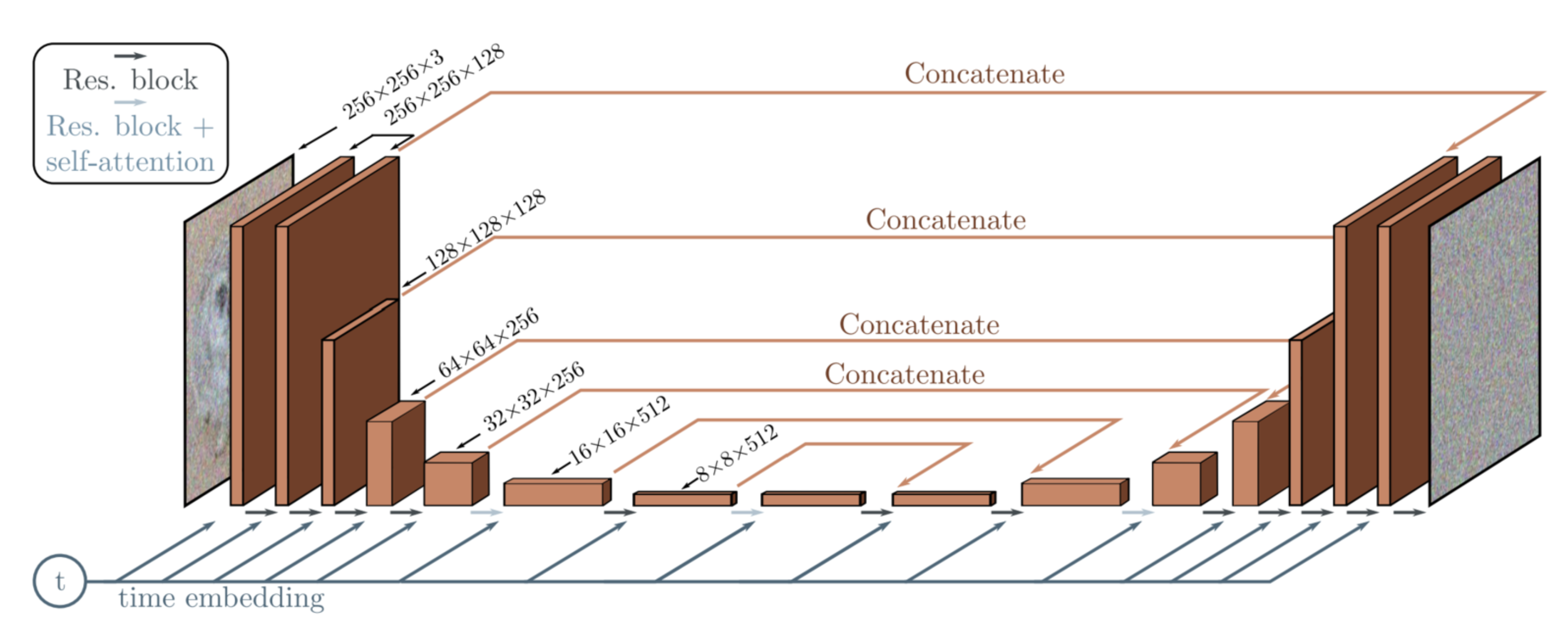
使用深度学习方法预测图像的噪声

预测图像噪声的神经网络模型有很多种，其中最常用的是 U-Net 结构。U-Net 之所以得名，是因为它的形状类似于字母“U”，具有对称的下采样（编码器）和上采样（解码器）路径，这两条路径通过跳跃连接（skip connections）相连，允许信息直接从编码器传递到解码器。除此之外，在 DDPM 的 U-Net 中，时间步 \(t\) 会经过一层嵌入层生成嵌入向量，然后通过卷积层与每一层的特征层相融合，最终得到预测的噪音。

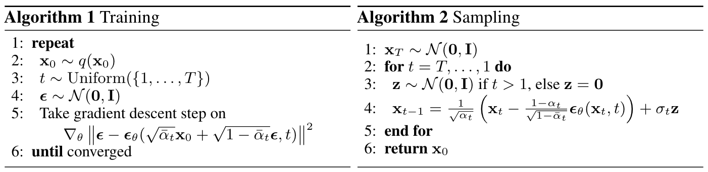
综上所属，模型的训练和去噪过程可以概括如下：